Efficient Partitioning of Road Networks

Design techniques based on classical algorithms have proved useful for recent innovation on several large-scale problems, such as travel itineraries and routing challenges. For example, Dijkstra’s algorithm is often used to compute routes in graphs, but the size of the computation can increase quickly beyond the scale of a small town. The process of "partitioning" a road network, however, can greatly speed up algorithms by effectively shrinking how much of the graph is searched during computation.

In this post, we cover how we engineered a graph partitioning algorithm for road networks using ideas from classic algorithms, parts of which were presented in “Sketch-based Algorithms for Approximate Shortest Paths in Road Networks” at WWW 2021. Using random walks, a classical concept that is counterintuitively useful for computing shortest routes by decreasing the network size significantly, our algorithm can find a high quality partitioning of the whole road network of the North American continent nearly an order of magnitude faster¹ than other partitioning algorithms with similar output qualities.

Using Graphs to Model Road Networks

There is a well-known and useful correspondence between road networks and graphs, where intersections become nodes and roads become edges.

Image from Wikipedia

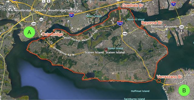
To understand how routing might benefit from partitioning, consider the most well-known solution for finding the fastest route: the Dijkstra algorithm, which works in a breadth-first search manner. The Dijkstra algorithm performs an exhaustive search starting from the source until it finds the destination. Because of this, as the distance between the source and the destination increases, the computation can become an order of magnitude slower. For example, it is faster to compute a route inside Seattle, WA than from Seattle, WA to San Francisco, CA. Moreover, even for intra-metro routes, the exhaustive volume of space explored by the Dijkstra algorithm during computation results in an impractical latency on the order of seconds. However, identifying regions that have more connections inside themselves, but fewer connections to the outside (such as Staten Island, NY) makes it possible to split the computation into multiple, smaller chunks.

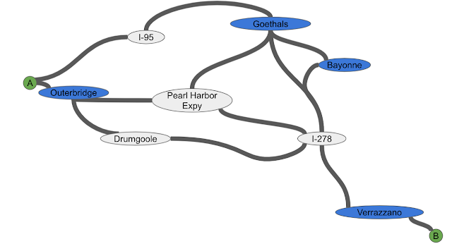
Top: A routing problem around Staten Island, NY. Bottom: Corresponding partitioning as a graph. Blue nodes indicate the only entrances to/exits from Staten Island.

Consider driving from point A to point B in the above image. Once one decides where to enter Staten Island (Outerbridge or Goethals) and where to exit (Verrazzano), the problem can be broken into the three smaller pieces of driving: To the entrance, the exit, and then the destination using the best route available. That means a routing algorithm only needs to consider these special points (beacons) to navigate between points A and B, and can thus find the shortest accurate path faster.

Note that beacons are only useful as long as there are not too many of them — the fewer beacons there are, the fewer shortcuts need to be added, the smaller the search space, and the faster the computation — so a good partitioning should have relatively fewer beacons for the number of components (i.e., a particular area of a road network).

As the example of Staten Island illustrates, real-life road networks have many beacons (special points, such as bridges, tunnels, or mountain passes) that result in some areas being very well connected (e.g., with large grids of streets) and others being poorly connected (e.g., an island only accessible via a couple of bridges). The question becomes how to efficiently define the components and identify the smallest number of beacons that connect the road network.

Our Partitioning Algorithm

Because each connection between two components is a potential beacon, the approach we take to ensure there are not too many beacons is to divide the road network in a way that minimizes the number of connections between components.

To do this, we start by dividing the network into two balanced (i.e., of similar size) components while also minimizing the number of roads that connect those two components, which results in an effectively small ratio of beacons to roads in each component. Then, the algorithm keeps dividing the network two at a time until all the components reach the desired size (in terms of the number of roads inside) that yields a useful multi-component partition. There is a careful balance here. If the size is too small, we will get too many beacons; whereas if it is too large, then it will be useful only for long routes. Therefore the size is left as an input parameter and found through experimentation when the algorithm is being finalized.

While there are numerous partitioning schemes, such as METIS (for general networks), PUNCH and inertial-flow (both optimized for road-like networks), our solution is based on the inertial-flow algorithm, augmented to run as efficiently on whole continents as it does on cities.

Balanced Partitioning for Road Networks

How does one divide a road network represented as a graph into two balanced components, as mentioned above? A first step is to make a graph smaller by grouping closely connected nodes together, which allows us to speed up the following two-way partitioning phase. This is where a random walk is useful.

Random walks enjoy many useful theoretical properties — which is why they have been used to study a range of topics from the motion of mosquitoes in a forest to heat diffusion — the most relevant for our application being that they tend to get “trapped” in regions that are well connected inside but poorly connected outside. Consider a random walk on the streets of Staten Island for a fixed number of steps: because relatively few roads exit the island, most of the steps happen inside the island, and the probability of stepping outside the island is low.

Illustration of a random walk. Suppose the blue graph is a hypothetical road network corresponding to Staten Island. 50 random walks are performed, all starting at the middle point. Each random walk continues for 10 steps or until it steps out of the island. The numbers at each node depict how many times they were visited by a random walk. By the end, any node inside the island is visited much more frequently than the nodes outside.

After finding these small components, which will be highly connected nodes grouped together (such as Staten Island in the above example), the algorithm contracts each group into a new, single node.

Reducing the size of the original graph (left) by finding groups of nodes (middle) and coalescing each group into a single “super” node (right). Example here chosen manually to better illustrate the rest of the algorithm.

The final steps of the algorithm are to partition this much smaller graph into two parts and then refine the partitioning on this small graph to one on the original graph of the road network. We then use the inertial flow algorithm to find the cut on the smaller graph that minimizes the ratio of beacons (i.e., edges being cut) to nodes.

The algorithm evaluates different directions. For each direction, we find the division that minimizes the number of edges cut (e.g., beacons) between the first and last 10% of the nodes

Having found a cut on the small graph, the algorithm performs a refinement step to project the cut back to the original graph of the road network.

Conclusion

This work shows how classical algorithms offer many useful tools for solving problems at large scale. Graph partitioning can be used to break down a large scale graph problem into smaller subproblems to be solved independently and in parallel — which is particularly relevant in Google maps, where this partitioning algorithm is used to efficiently compute routes.

Acknowledgements

We thank our collaborators Lisa Fawcett, Sreenivas Gollapudi, Kostas Kollias, Ravi Kumar, Andrew Tomkins, Ameya Velingker from Google Research and Pablo Beltran, Geoff Hulten, Steve Jackson, Du Nguyen from Google Maps.

¹This technique can also be used for any network structure, such as that for brain neurons. ^↩