Bi-Tempered Logistic Loss for Training Neural Nets with Noisy Data

The quality of models produced by machine learning (ML) algorithms directly depends on the quality of the training data, but real world datasets typically contain some amount of noise that introduces challenges for ML models. Noise in the dataset can take several forms from corrupted examples (e.g., lens flare in an image of a cat) to mislabelled examples from when the data was collected (e.g., an image of cat mislabelled as a flerken).

The ability of an ML model to deal with noisy training data depends in great part on the loss function used in the training process. For classification tasks, the standard loss function used for training is the logistic loss. However, this particular loss function falls short when handling noisy training examples due to two unfortunate properties:

1. Outliers far away can dominate the overall loss: The logistic loss function is sensitive to outliers. This is because the loss function value grows without bound as the mislabelled examples (outliers) are far away from the decision boundary. Thus, a single bad example that is located far away from the decision boundary can penalize the training process to the extent that the final trained model learns to compensate for it by stretching the decision boundary and potentially sacrificing the remaining good examples. This “large-margin” noise issue is illustrated in the left panel of the figure below.
2. Mislabeled examples nearby can stretch the decision boundary: The output of the neural network is a vector of activation values, which reflects the margin between the example and the decision boundary for each class. The softmax transfer function is used to convert the activation values into probabilities that an example will belong to each class. As the tail of this transfer function for the logistic loss decays exponentially fast, the training process will tend to stretch the boundary closer to a mislabeled example in order to compensate for its small margin. Consequently, the generalization performance of the network will immediately deteriorate, even with a low level of label noise (right panel below).

We visualize the decision surface of a 2-layered neural network as it is trained for binary classification. Blue and orange dots represent the examples from the two classes. The network is trained with logistic loss under two types of noisy conditions: (left) large-margin noise and (right) small-margin-noise.

We tackle these two problems in a recent paper by introducing a “bi-tempered” generalization of the logistic loss endowed with two tunable parameters that handle those situations well, which we call “temperatures”—t₁, which characterizes boundedness, and t₂ for tail-heaviness (i.e. the rate of decline in the tail of the transfer function). These properties are illustrated below. Setting both t₁ and t₂ to 1.0 recovers the logistic loss function. Setting t₁ lower than 1.0 increases the boundedness and setting t₂ greater than 1.0 makes for a heavier-tailed transfer function. We also introduce this interactive visualization which allows you to visualize the neural network training process with the bi-tempered logistic loss.

Left: Boundedness of the loss function. When t1 is between 0 and 1, exclusive, only a finite amount of loss is incurred for each example, even if they are mislabeled. Shown is t1 = 0.8. Right: Tail-heaviness of the transfer function. The heavy-tailed transfer function applies when t2 = > 1.0 and assigns higher probability for the same amount of activation, thus preventing the boundary from drawing closer to the noisy example. Shown is t2 = 2.0.

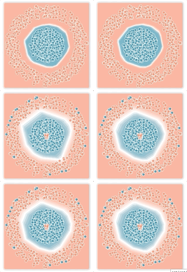
To demonstrate the effect of each temperature, we train a two-layer feed-forward neural network for a binary classification problem on a synthetic dataset that contains a circle of points from the first class, and a concentric ring of points from the second class. You can try this yourself on your browser with our interactive visualization. We use the standard logistic loss function, which can be recovered by setting both temperatures equal to 1.0, as well as our bi-tempered logistic loss for training the network. We then demonstrate the effects of each loss function for a clean dataset, a dataset with small-margin noise, large-margin noise, and a dataset with random noise.

Logistic vs. bi-tempered logistic loss: (a) noise-free labels, (b) small-margin label noise, (c) large-margin label noise, and (d) random label noise. The temperature values (t1, t2) for the tempered loss are shown above each figure. We find that for each situation, the decision boundary recovered by training with the bi-tempered logistic loss function is better than before.

Noise Free Case:
We show the results of training the model on the noise-free dataset in column (a), using the logistic loss (top) and the bi-tempered logistic loss (bottom). The white line shows the decision boundary for each model. The values of (t₁, t₂), the temperatures in the bi-tempered loss function, are shown below each column of the figure. Notice that for this choice of temperatures, the loss is bounded and the transfer function is tail-heavy. As can be seen, both losses produce good decision boundaries that successfully separates the two classes.

Small-Margin Noise:
To illustrate the effect of tail-heaviness of the probabilities, we artificially corrupt a random subset of the examples that are near the decision boundary, that is, we flip the labels of these points to the opposite class. The results of training the networks on data with small-margin noise using the logistic loss as well as the bi-tempered loss is shown in column (b).

As can be seen, the logistic loss, due to the lightness of the softmax tail, stretches the boundary closer to the noisy points to compensate for their low probabilities. On the other hand, the bi-tempered loss using only the tail-heavy probability transfer function by adjusting t₂ can successfully avoid the noisy examples. This can be explained by the heavier tail of the tempered exponential function, which assigns reasonably high probability values (and thus, keeps the loss value small) while maintaining the decision boundary away from the noisy examples.

Large-Margin Noise:
Next, we evaluate the performance of the two loss functions for handling large-margin noisy examples. In (c), we randomly corrupt a subset of the examples that are located far away from the decision boundary, the outer side of the ring as well as points near the center).

For this case, we only use the boundedness property of the bi-tempered loss, while keeping the softmax probabilities the same as the logistic loss. The unboundedness of the logistic loss causes the decision boundary to expand towards the noisy points to reduce their loss values. On the other hand, the bounded bi-tempered loss, bounded by adjusting t₁, incurs a finite amount of loss for each noisy example. As a result, the bi-tempered loss can avoid these noisy examples and maintain a good decision boundary.

Random Noise:
Finally, we investigate the effect of random noise in the training data on the two loss functions. Note that random noise comprises both small-margin and large-margin noisy examples. Thus, we use both boundedness and tail-heaviness properties of the bi-tempered loss function by setting the temperatures to (t₁, t₂) = (0.2, 4.0).

As can be seen from the results in the last column, (d), the logistic loss is highly affected by the noisy examples and clearly fails to converge to a good decision boundary. On the other hand, the bi-tempered can recover a decision boundary that is almost identical to the noise-free case.

Conclusion
In this work we constructed a bounded, tempered loss function that can handle large-margin outliers and introduced heavy-tailedness in our new tempered softmax function, which can handle small-margin mislabeled examples. Using our bi-tempered logistic loss, we achieve excellent empirical performance on training neural networks on a number of large standard datasets (please see our paper for full details). Note that the state-of-the-art neural networks have been optimized along with a large variety of variables such as: architecture, transfer function, choice of optimizer, and label smoothing to name just a few. Our method introduces two additional tunable variables, namely (t₁, t₂). We believe that with a systematic “joint optimization” of all commonly tried variables, significant further improvements can be achieved in conjunction with our loss function. This is of course a more long-term goal. We also plan to explore the idea of annealing the temperature parameters over the training process.

Acknowledgements:
This blogpost reflects work with our co-authors Manfred Warmuth, Visiting Researcher and Tomer Koren, Senior Research Scientist, Google Research. Preprint of our paper is available here, which contains theoretical analysis of the loss function and empirical results on standard datasets at scale.