Learning Better Simulation Methods for Partial Differential Equations

The world’s fastest supercomputers were designed for modeling physical phenomena, yet they still are not fast enough to robustly predict the impacts of climate change, to design controls for airplanes based on airflow or to accurately simulate a fusion reactor. All of these phenomena are modeled by partial differential equations (PDEs), the class of equations that describe everything smooth and continuous in the physical world, and the most common class of simulation problems in science and engineering. To solve these equations, we need faster simulations, but in recent years, Moore’s law has been slowing. At the same time, we’ve seen huge breakthroughs in machine learning (ML) along with faster hardware optimized for it. What does this new paradigm offer for scientific computing?

In “Learning Data Driven Discretizations for Partial Differential Equations”, published in Proceedings of the National Academy of Sciences, we explore a potential path for how ML can offer continued improvements in high-performance computing, both for solving PDEs and, more broadly, for solving hard computational problems in every area of science.

For most real-world problems, closed-form solutions to PDEs don’t exist. Instead, one must find discrete equations (“discretizations”) that a computer can solve to approximate the continuous PDE. Typical approaches to solve PDEs represent equations on a grid, e.g., using finite differences. To achieve convergence, the mesh spacing of the grid needs to be smaller than the smallest feature size of the solutions. This often isn’t feasible because of an unfortunate scaling law: achieving 10x higher resolution requires 10,000x more compute, because the grid must be scaled in four dimensions—three spatial dimensions and time. Instead, in our paper we show that ML can be used to learn better representations for PDEs on coarser grids.

Satellite photo of a hurricane, at both full resolution and simulated resolution in a state-of-the-art weather model. Cumulus clouds (e.g., in the red circle) are responsible for heavy rainfall, but in the weather model the details are entirely blurred out. Instead, models rely on crude approximations for sub-grid physics, a key source of uncertainty in climate models. Image credit: NOAA

The challenge is to retain the accuracy of high-resolution simulations while still using the coarsest grid possible. In our work we’re able to improve upon existing schemes by replacing heuristics based on deep human insight (e.g., “solutions to a PDE should always be smooth away from discontinuities”) with optimized rules based on machine learning. The rules our ML models recover are complex, and we don’t entirely understand them, but they incorporate sophisticated physical principles like the idea of “upwinding”—to accurately model what’s coming towards you in a fluid flow, you should look upstream in the direction the wind is coming from. An example of our results on a simple model of fluid dynamics are shown below:

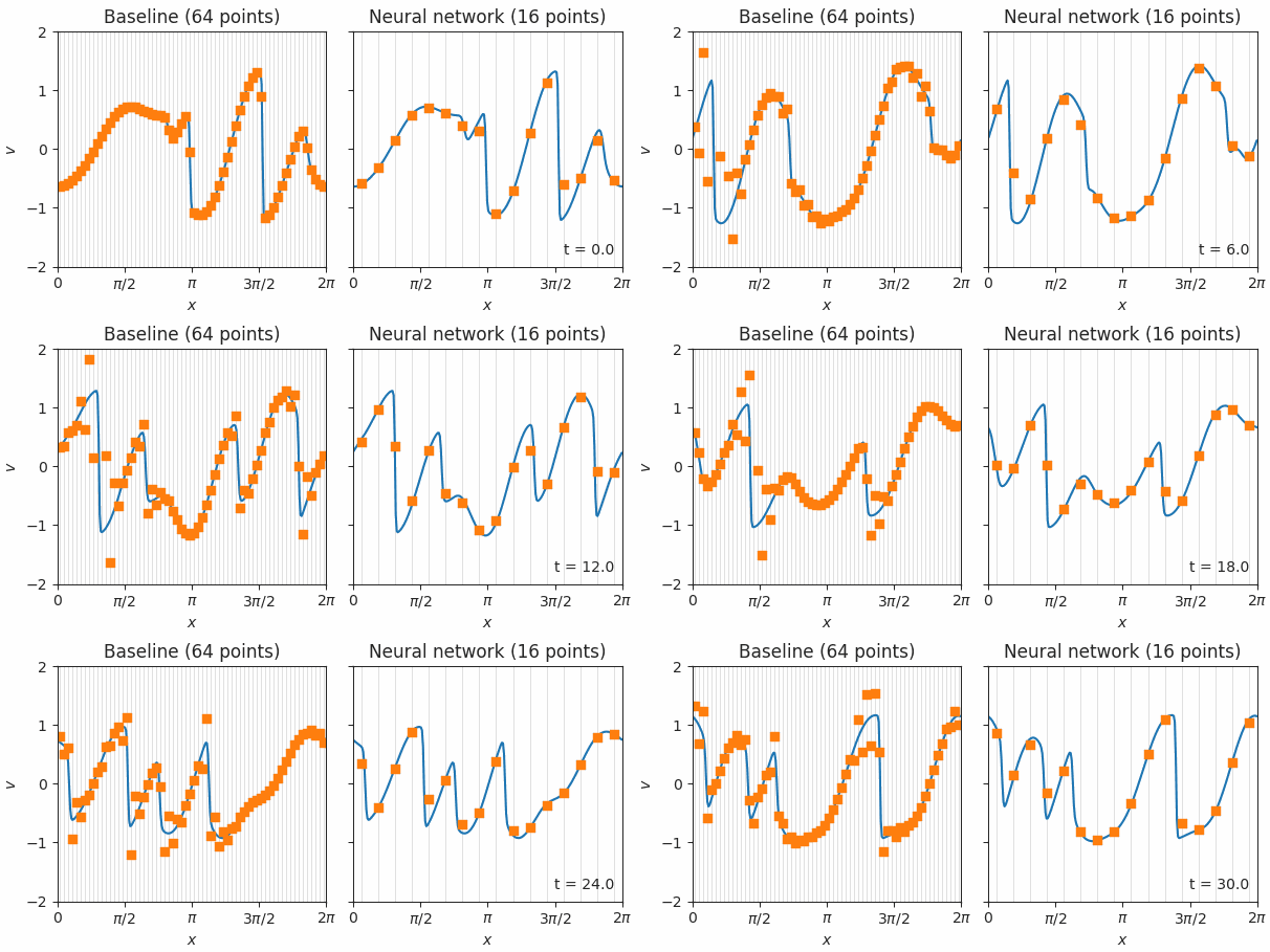
Simulations of Burgers’ equation, a model for shock waves in fluids, solved with either a standard finite volume method (left) or our neural network based method (right). The orange squares represent simulations with each method on low resolution grids. These points are fed back into the model at each time step, which then predicts how they should change. Blue lines show the exact simulations used for training. The neural network solution is much better, even on a 4x coarser grid, as indicated by the orange squares smoothly tracing the blue line.

Our research also illustrates a broader lesson about how to effectively combine machine learning and physics. Rather than attempting to learn physics from scratch, we combined neural networks with components from traditional simulation methods, including the known form of the equations we’re solving and finite volume methods. This means that laws such as conservation of momentum are exactly satisfied, by construction, and allows our machine learning models to focus on what they do best, learning optimal rules for interpolation in complex, high-dimensional spaces.

Next Steps
We are focused on scaling up the techniques outlined in our paper to solve larger scale simulation problems with real-world impacts, such as weather and climate prediction. We’re excited about the broad potential of blending machine learning into the complex algorithms of scientific computing.

Acknowledgments
Thanks to co-authors Yohai Bar-Sinari, Jason Hickey and Michael Brenner; and Google collaborators Peyman Milanfar, Pascal Getreur, Ignacio Garcia Dorado, Dmitrii Kochkov, Jiawei Zhuang and Anton Geraschenko.